DTI
DTI
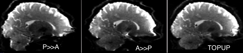
This page assumes you familiar with the ideas described of diffusion tensor imaging (see my class for details), so you may want to read that first. This advanced page describes how FSL’s topup can be used to undistort diffusion images, and provides a matlab script for batch processing large numbers of images with topup and FDT. Topup does an incredible job unwarping images, but the current beta form involves a lot of steps and knowledge about your dataset. This script will automatically detect and separate the B0 images required by topup, simplifying topup. The effects are shown in the images on the left: the top row shows a distorted image, the middle row shows an image distorted in the opposite direction, and the bottom rom shows the pair combined after undistrotion.
Undistorting DTI Data
Diffusion images are acquired rapidly, and slices are typically acquired using 2D sequences (usually Echo Planar Imaging [EPI]) that acquire an entire 2D slice in a single excitation. Unfortunately, these sequences take a while to read-out the slice, and therefore any field homogeneity errors will cause spatial distortion. While scanner shimming aims to reduce field inhomogeneity, the solutions will be imperfect, particularly where there are different types of tissue present – for the brain this is particularly the sinuses near the orbital frontal cortex and regions near the ear canals. While these distortions are inevitable, we can compensate for them by acquiring two series of images that have opposite phase-encoding direction but identical in all other respects. Each of these images will end up showing distortions of identical magnitude, but opposite direction. Topup compares these two images to the nonlinear midpoint deformation between these two images. The deformation can then be applied to all the images, creating a combined image with minimal spatial distortion. Topup calculates these deformations based on the B0 images (as these are not contaminated by additional eddy current deformations of the directional scans), and then computes a mean image for each pair (positive and negative polarity) of images (so that both the B0 and directional scans are corrected). Therefore the two input series (positive and negative) create a single unwarped series that should have 1.4 times the signal to noise of either original (thanks to signal averaging).
When you run my script ‘ dti_1_eddy ’ it expects to to provide positive and negative polarity images (these should be 4D NIfTI format images). For example, if your anterior-to-postrior phased-encoded image is named named “AP.nii” and the posterior-to-anterior image is named “PA.nii” you would run something like ‘./dti_1_eddy.sh “AP” “PA”’. If all works well, the script will run TOPUP followed by Eddy. If you only provide a since image (‘./dti_1_edyy “PA.nii”’) the script will run the legacy eddy_correct (which only does a linear spatial correction). Note that users who have a graphics card set up for CUDA as well as a CUDA-capable version of FSL’s Eddy, there is a much faster way to do the same thing: my script ‘dti_1_eddy_cuda’.
Notes
By default, most Philips and GE scanners use a monopolar Stejskal-Tanner sequence, while most Siemens use a bipolar ` twice-refocused spin echo <https://pubmed.ncbi.nlm.nih.gov/12509835>`_ sequence. The bipolar sequences show less distortion and are less sensitive to background gradients. The monopolar sequences are able to have more signal thanks to a shorter TE. Users of bipolar sequences will see less benefit of topup. Siemens users who want to use monopolar DTI can install the Multi-Band Accelerated Pulse Sequences (even if you do not use multiband features, these sequences allow you to choose between monopolar or bipolar). These sequences are really impressive, though you may want to tune the protocols for your scanner (centers with 32-channel headcoils may want to look at the protocols Multiband Imaging Test-Retest Pilot Dataset ). Setting up DTI sequences is challenging, and may be specific for your scanners (e.g. for the Siemens Trio avoid echo spacing in the range of 0.59 ms to 0.70 ms to minimize harmonic vibrations).
By default, most scanners only acquire a single B0 image when acquiring DTI – for example a 32 direction scan will have 33 volumes, with the first being the B0 scan. However, it is often advisable to make sure that about 1/10th of your images are B0 scans, as this will provide more accurate ADC/MD estimates as well as better topup estimates. For Siemens scanners you can create custom DiffusionVectors.txt that specify any number of gradient directions ( online tools calculate optimal directions ) and you can add extra B0 scans by inserting directions with the vector “0 0 0” at regular intervals. You can also use the command line tool ‘gps’ that is included with FSL .
Topup requires you to specify the readout time of your image. However, as long as this is identical for all your scans (and it typically is), you do not have to be precise about this value. In the case where the readout is identical for all scans an incorrect readout time will simply result in an error in the scale of the calibrated fieldmap (topup will assume the shim was better or worse than reality), but the undistortion will be identical. Since we usually acquire spin-echo DTI images with the minimum possible echo time, the readout time will be somewhat less than the echo time (TE). Consider our example DTI scan with a TE of 79.2ms – the refocusing pulse occurs at 39.6ms and so we cannot begin reading out until after 39.6ms and therefore must end by 118.8 ms (for a mean TE of 79.2ms). To precisely calculate the time you will want to compute readOutTime = echoSpacing * ((matrixLines*partialFourier/accelerationFactor)-1). You can find the echo spacing on the ‘Sequence’ tab of the Siemens scanner (referred to as ‘dwell time’ by some). For our example dataset the echoSpacing = 0.77ms (0.00077s), we have 90 lines of data acquired with full Fourier (partialFourier=1) and GRAPPA=2 (accelerationFactor = 2), so the readout time is 0.03388 seconds (= 0.00077 * ((90*0.5)-1). I strongly suggestion you look at the FSL eddy web page for hints on setting up your sequence.
29 May 2013. Chris Rorden with suggestions from Dirk den Ouden and Svetlana Malyutina